Project 3: Molecular Dynamics Short-Range Force Computation — CPU Performance Optimization
0. Getting Started
Project 3 is a Coding Project, so you should accept your homework via GitHub Classroom link first. This repository has starter code template.
For convenience, this year we offer you a unified Online Judge with SSH protocal. You can see below instructions to set up. But you SHOULD ALSO push to GitHub and then submit to Gradescope. We will review your code through Gradescope platform. But we'll use rejudge on SOJ, and use this result as final score.
IMPORTANT NOTICE
In order to improve your AI skills for coding, this year, we
canceled Top-30 score, and allows you to use
AI for any exploration. But we WILL ALSO check
plagiarism. And for those who're at top-30 speed up ratio or if
you receieved a request, you should submit your
WriteUp to
hezb2023<at>shanghaitech.edu.cn and
hanlt2025<at>shanghaitech.edu.cn. If you're
using AI, please attach your complete AI
conversation flow below. We'll check carefully and share some
good ideas or writeups after this project for you all to
study!
1. Physics Background
1.1 Lennard-Jones Potential
Molecular Dynamics (MD) simulation numerically evolves the trajectories of a large number of particles by solving Newton's equations of motion. It is a core method in computational chemistry, materials science, and biophysics (software packages such as GROMACS, LAMMPS, and NAMD consume billions of CPU core-hours worldwide every day).
Lennard-Jones (LJ) potential is the most classical model for describing non-bonded interactions (van der Waals forces + short-range repulsion):
where:
- is the distance between two particles
- determines the equilibrium distance (the potential energy minimum is at )
- is the well depth
- The 12th-power term describes short-range electron cloud repulsion
- The 6th-power term describes long-range attraction (London dispersion force)
This project uses reduced units: , thus
1.2 Scalar Form of Force
The force on particle due to particle (along the direction ):
Let , then .
Newton's third law guarantees .
1.3 Cutoff and Periodic Boundary Conditions (PBC)
Computing interactions for all particle pairs is prohibitively expensive. Physically, the LJ potential decays very rapidly for (approximately 1.6% of ), so cutoff is adopted in all mainstream MD packages:
To simulate an infinite system, periodic boundary conditions are used: particles reside in a cubic box of side length , and each particle's "image copies" periodically tile all of space. The distance between two particles follows the minimum image convention:
1.4 Cell List Acceleration to
The box is uniformly divided into cells with side length . All neighbors within the cutoff distance of a given particle must be in its own cell or the 26 adjacent cells. The computational complexity drops from to (linear!), at the cost of a more complex data structure.
The baseline provided in this project already implements a cell list, but it is inefficient (no SIMD/OpenMP) and awaits your optimization.
2. Task Definition
Implement the function:
void compute_forces_optimized(ParticleSystem *sys);Input: sys already contains
filled pos[N] (particle positions), n
(number of particles), box (box side length)
Output: Fill sys->force[N]
so that the net force on each particle satisfies a relative
error
(compared with the baseline)
Constraints:
- Do not use numerical libraries such as BLAS / FFTW / Intel MKL
- You may only modify
src/optimized.cand thenumactlconfiguration file (see below); all other modifications will be ignored - Do not attack or forge data
3. Input Parameters
init_particles(N, density, seed) places
particles in a cubic box of
:
- Box side length , where is the density (default 0.5)
- Initial particle positions: placed on a cubic lattice with spacing + 10% Gaussian jitter (to avoid divergent forces from overlapping particles)
- Force conservation: theoretically (the evaluation will check this)
Evaluation scales:
For each size
,
bench.sh records one measured baseline time
without a baseline warmup. It records the best optimized time
over 5 measured runs, after one optimized warmup. The per-size
speedup is:
The final score uses the geometric mean of the per-size speedups:
bench.sh computes GeoSpeedup from
the full-precision per-size ratios and rounds only the printed
result to two decimals. This is equivalent to
,
but the log form is more numerically stable.
4. Local Testing
4.1 Build
make # Compile all binaries into bin/4.2 Correctness Verification
make correctness    # brute-force vs baseline, small scale (512, 1000, 2000)
make test N=4096    # baseline vs optimized, check force error < 1e-6
4.3 Performance Benchmark
./bench.shExample output:
=== N-body Benchmark ===
Sizes=2000000 4000000 8000000  density=0.5  seed=42  optimized_runs=5 (+ optimized warmup per size)

===============================
N=2000000  density=0.5  seed=42  baseline_runs=1  optimized_runs=5 (+ optimized warmup)

[1 - Baseline]
  Run 1  : 1.234 s
  Time   : 1.234 s

[2 - Optimized]
  Warmup : done
  Run 1  : 0.456 s
  ...
  Best   : 0.440 s

[3] Correctness
...

-------------------------------
  N         : 2000000
  Baseline  : 1.234 s (single run)
  Optimized : 0.440 s (best of 5)
  Speedup   : 2.80x
-------------------------------

...

===============================
GeoSpeedup : 2.75x
Sizes      : 2000000 4000000 8000000
===============================
4.4 Common Development Commands
| Command | Description |
|---|---|
make |
Build everything |
make correctness |
Small-scale correctness verification |
make test N=... |
Baseline vs optimized force comparison |
make clean |
Clean bin/, tmp/,
src/*.o |
cd src && make |
Quick compile check (-O0 -g, for
debugging) |
5. Submitting to the Evaluation System
Evaluation is conducted via SOJ (SSH-protocol Online Judge).
5.0 Adding SSH Public Key on Github
In the terminal, run ssh-keygen and press Enter
throughout.
This will generate two files. Taking
/home/zambar/.ssh/id_ed25519 as an example, this is
your private key—please keep it safe and never share it
anywhere! And /home/zambar/.ssh/id_ed25519.pub is
your public key.
Go to https://github.com/settings/keys,
click New SSH Key, and paste your public key into
the content field.
After completing the addition, ensure that running the following command locally returns normally:
ssh -T git@github.comIf it returns something like:
Hi HeZeBang! You've successfully authenticated, but GitHub does not provide shell access.Then the configuration is successfully set up.
5.1 Configure SSH
Add the following to ~/.ssh/config:
Host soj
    HostName 10.15.89.111
    Port 2222
    User [Your_Github_UserName]
Test the connection:
ssh sojYou should see the SOJ welcome message and available command prompts.
5.2 Upload Files
You need to upload two files using scp (path
format: <problemID>/<filename>):
# Upload optimized code
scp src/optimized.c soj:proj3/optimized.c

# Upload affinity configuration
scp affinity.conf soj:proj3/affinity.confNote: If
scpreports an error, it may be due to OpenSSH version differences:
< 8.7: Use thesftpcommand instead8.7 ~ 9.0: Add the-soption, e.g.,scp -s ...> 9.0: Works directly
5.3 Submit for Evaluation
After uploading, trigger the evaluation in the SSH shell:
ssh soj submit proj3Check submission status:
ssh soj list          # List all submissions
ssh soj status <id>   # View details of a specific submission
5.4 affinity.conf Description
To provide the most realistic tuning experience, we allow you
to modify numactl runtime parameters via a
configuration file. You can look up relevant documentation to
understand how this works and how to optimize your program's
execution.
affinity.conf controls how numactl
binds CPUs/memory. The format is key = value, one
entry per line:
# CPU binding (choose at most one)
physcpubind = 0-127         # Specify physical CPU range
cpunodebind = 0             # Specify NUMA node

# Memory binding (choose at most one)
membind     = 0             # Only allocate from specified node
interleave  = 0,1           # Round-robin allocation across nodes
preferred   = 0             # Prefer a node, but allow spillover
localalloc  = true          # Allocate on the node where the CPU resides
Leave empty to disable numactl, letting the
kernel scheduler choose CPUs. See
affinity.conf.example for reference.
6. Grading Criteria
Scores are computed based on the geometric mean speedup using piecewise linear interpolation:
| Speedup (GeoSpeedup) | Score |
|---|---|
| 0x | 0% |
| 1x | 20% |
| 10x | 30% |
| 20x | 40% |
| 30x | 50% |
| 40x | 60% |
| 50x | 80% |
| 85x+ | 100% |
Between key points, the score is linearly interpolated. Examples:
- 5x speedup → 25% (midpoint between 1x at 20% and 10x at 30%)
- 15x speedup → 35% (midpoint between 10x at 30% and 20x at 40%)
Compilation error or wrong answer results in 0 points regardless of speedup.
7. Appendix
Evaluation Machine Specifications
Both our submission server and final evaluation machine run on this AMD EPYC machine, so the following information may be helpful.
lscpu
Architecture:                            x86_64
CPU op-mode(s):                          32-bit, 64-bit
Address sizes:                           43 bits physical, 48 bits virtual
Byte Order:                              Little Endian
CPU(s):                                  128
On-line CPU(s) list:                     0-127
Vendor ID:                               AuthenticAMD
Model name:                              AMD EPYC 7742 64-Core Processor
CPU family:                              23
Model:                                   49
Thread(s) per core:                      1
Core(s) per socket:                      64
Socket(s):                               2
Stepping:                                0
Frequency boost:                         enabled
CPU max MHz:                             2250.0000
CPU min MHz:                             1500.0000
BogoMIPS:                                4500.19
Flags:                                   fpu vme de pse tsc msr pae mce cx8 apic sep mtrr pge mca cmov pat pse36 clflush mmx fxsr sse sse2 ht syscall nx mmxext fxsr_opt pdpe1gb rdtscp lm constant_tsc rep_good nopl nonstop_tsc cpuid extd_apicid aperfmperf rapl pni pclmulqdq monitor ssse3 fma cx16 sse4_1 sse4_2 movbe popcnt aes xsave avx f16c rdrand lahf_lm cmp_legacy svm extapic cr8_legacy abm sse4a misalignsse 3dnowprefetch osvw ibs skinit wdt tce topoext perfctr_core perfctr_nb bpext perfctr_llc mwaitx cpb cat_l3 cdp_l3 hw_pstate ssbd mba ibrs ibpb stibp vmmcall fsgsbase bmi1 avx2 smep bmi2 cqm rdt_a rdseed adx smap clflushopt clwb sha_ni xsaveopt xsavec xgetbv1 xsaves cqm_llc cqm_occup_llc cqm_mbm_total cqm_mbm_local clzero irperf xsaveerptr rdpru wbnoinvd amd_ppin arat npt lbrv svm_lock nrip_save tsc_scale vmcb_clean flushbyasid decodeassists pausefilter pfthreshold avic v_vmsave_vmload vgif v_spec_ctrl umip rdpid overflow_recov succor smca sme sev sev_es ibpb_exit_to_user
Virtualization:                          AMD-V
L1d cache:                               4 MiB (128 instances)
L1i cache:                               4 MiB (128 instances)
L2 cache:                                64 MiB (128 instances)
L3 cache:                                512 MiB (32 instances)
NUMA node(s):                            2
NUMA node0 CPU(s):                       0-63
NUMA node1 CPU(s):                       64-127
Core-to-Core Latency
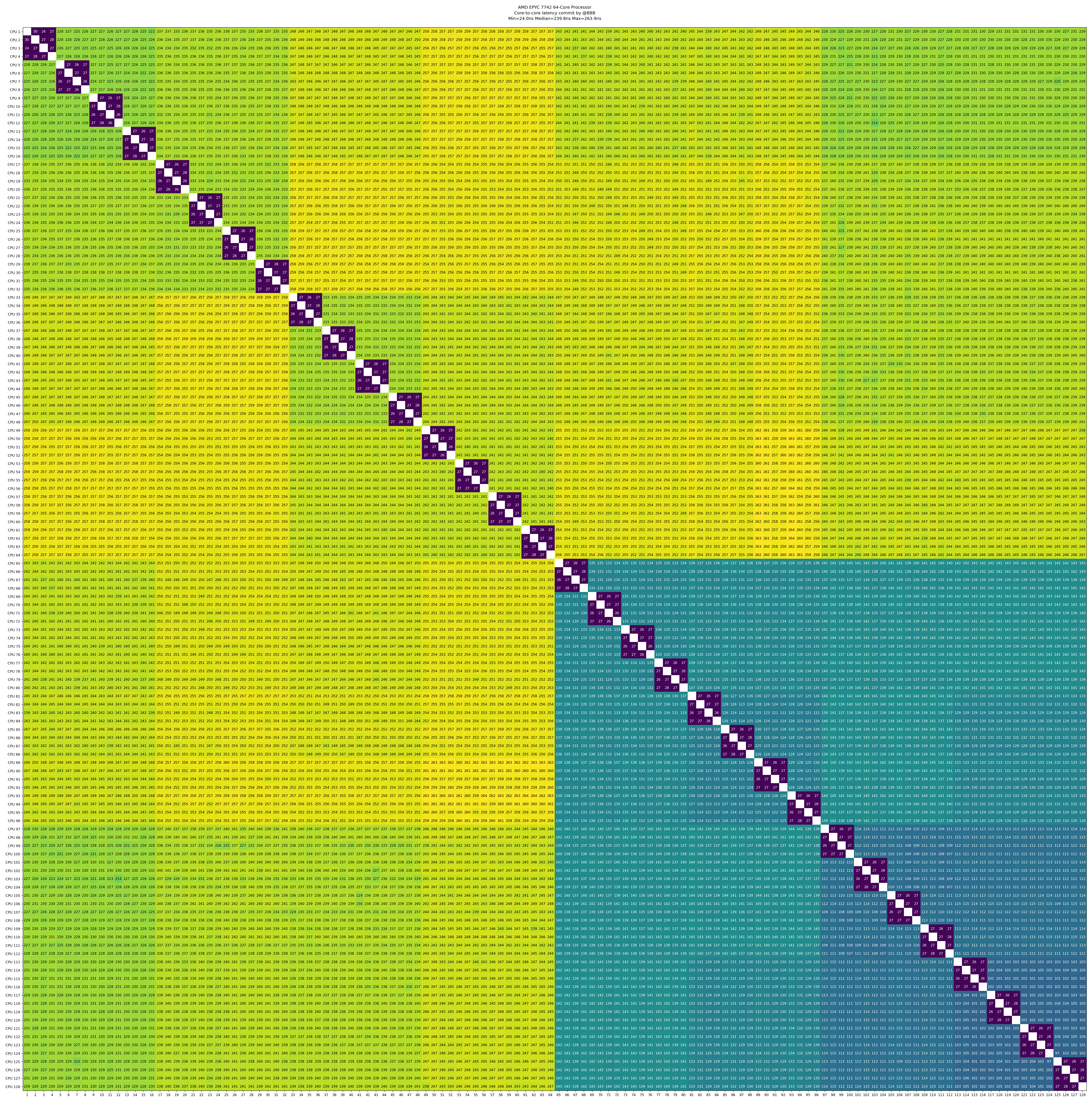
Topology

If you have questions about the problem or evaluation machine, you can contact:
- Any course instructor
hezb2023<at>shanghaitech.edu.cnhanlt2025<at>shanghaitech.edu.cn